4 Cross sections and decay rates

To be able to compare our calculated amplitudes to experimental data, we need to a bit more work. We have (142)

\displaystyle P_{i\to f}\sim\big{|}\langle{f}|\mathcal{S}|{i}\rangle|^{2}% \stackrel{{\scriptstyle i\neq f}}{{=}}\Big{(}(2\pi)^{4}\delta^{(4)}(P_{i}-P_{f% })\Big{)}^{2}\ \big{|}\langle{f}|\mathcal{T}|{i}\rangle\big{|}^{2}\,.

(230)

The squared delta function is a problem because we only need one of them to solve our integration; the other delta function will then automatically lead to yet another $\delta^{(4)}(0)$ . However, we have dealt with this problem before and know to write $(2\pi)^{4}\delta^{(4)}(0)=V$ with the volume of spacetime $V$ . Therefore, we instead consider the probability per volume $P/V$ . We also need to keep in mind that the states require a normalisation $1/\sqrt{E}$ . This leads to the probability density

\displaystyle\frac{{\rm d}P_{i\to f}}{V}=(2\pi)^{4}\delta^{(4)}(P_{i}-P_{f})\ % \big{|}\langle{f}|\mathcal{T}|{i}\rangle\big{|}^{2}\Bigg{(}\prod_{n=1}^{f}% \frac{{\rm d}^{3}p_{n}}{(2\pi)^{3}2E_{n}}\Bigg{)}\Bigg{(}\prod_{n=1}^{i}\frac{% 1}{2E_{n}}\Bigg{)}\,.

(231)

4.1 Two initial states: cross section

Many particle physics experiments are scattering experiments where we take two particles and collide them. In analogy to classical scattering, we define the cross section of the scattering. Since we are working in a quantum theory rather than a classical one, the cross section describes a probability rather than a physical size.

Consider a cloud of particles of type $a$ at rest with number density $\rho_{a}$ . Now we shoot a bunch of particles of (a potentially different) type $b$ at the cloud (cf. Figure 3). Along the axis of collision, we have a cross-sectional area $A$ and bunch lengths $l_{a}$ and $l_{b}$ . The cross section of the scattering is defined through the number $N$ of scattering events as

\displaystyle\sigma=\frac{N}{(\rho_{a}l_{a})(\rho_{b}l_{b})A}=N\underbrace{% \frac{A}{N_{a}\cdot N_{b}}}_{L^{-1}}\,.

(232)

Here we have also defined the total number of $a$ ( $b$ ) particles $N_{a}$ ( $N_{b}$ ). The combination $N_{a}N_{b}/A$ is called the luminosity and it is the reason that the cross section $\sigma$ is a useful quantity. If we were to repeat our $a$ - $b$ scattering experiment at a different collider which has e.g. more particles in its beams, we would see more events even though the underlying process has not changed. $\sigma$ encodes the physics, $L$ the parameters of the experiment. This allows us to focus on two-particle scattering and set $\rho_{a}=\rho_{b}=1$ even if the real beams may contain as many as $10^{11}$ particles (the beam intensity of the LHC beams).

A cloud of length la comprised of particles a is at rest. A second cloud (a beam) of type b and length lb is moving in to collide with the first cloud. The beam's cross-sectional area is A — Figure 3: A beam of particles of type $b$ is shot at a cloud of particles of type $a$ . The beam has length $l_{b}$ and the target $l_{a}$ . The cross sectional area of the target being hit by the beam is $A$ .

For a $2\to f$ process of momenta $p_{a},p_{b}\to p_{1},...,p_{f}$ , we have from (231)

\displaystyle\frac{{\rm d}P_{a,b\to f}}{V}=\frac{1}{(2E_{a})(2E_{b})}(2\pi)^{4% }\delta^{(4)}(P_{i}-P_{f})\ \big{|}\langle{f}|\mathcal{T}|{a,b}\rangle\big{|}^% {2}\Bigg{(}\prod_{n=1}^{f}\frac{{\rm d}^{3}p_{n}}{(2\pi)^{3}2E_{n}}\Bigg{)}\,.

(233)

Keep in mind that the volume here is the spacetime volume of the scattering, i.e. $V=t\cdot A\cdot l_{a}$ . For a single scattering, the probability $P$ is the number of scattered particles. Therefore the cross section

\displaystyle{\rm d}\sigma=\frac{{\rm d}P_{a,b\to f}}{l_{a}\,l_{b}\,A}=\frac{{% \rm d}P_{a,b\to f}}{V}\frac{t}{l_{b}}\,.

(234)

Identifying $l_{b}/t$ as the velocity of the beam relative to our cloud of particles $a$ , we can now write

\displaystyle{\rm d}\sigma=\frac{{\rm d}P_{a,b\to f}}{V|\vec{v}|}=\frac{1}{(2E% _{a})(2E_{b})|\vec{v}|}\underbrace{\Bigg{(}\prod_{n=1}^{f}\frac{{\rm d}^{3}p_{% n}}{(2\pi)^{3}2E_{n}}\Bigg{)}(2\pi)^{4}\delta^{(4)}\Bigg{(}p_{a}+p_{b}-\sum_{n% =1}^{f}p_{n}\Bigg{)}}_{{\rm d}\Phi_{2\to f}}\ \underbrace{\big{|}\langle{f}|% \mathcal{T}|{a,b}\rangle\big{|}^{2}}_{|\mathcal{M}(a,b\to f)|^{2}}\,.

(235)

We now need to convince ourselves that ${\rm d}\sigma$ is Lorentz invariant since we could otherwise stop a process from happening simply by moving relative to it. We have already seen that the measure ${\rm d}^{3}p/(2E)$ is invariant, making the entire phase space ${\rm d}\Phi$ Lorentz invariant. The matrix element $\mathcal{M}(a,b\to f)$ is also fine so that the remaining part is the flux factor $E_{a}E_{b}|\vec{v}|$ . We an rewrite this in terms of invariants⁷⁷ 7 Note that technically this is only invariant for boosts along the beam axis. For boosts along any other axis, it is not invariant which fits well with our intuition of cross-sectional areas.

\displaystyle E_{a}E_{b}|\vec{v}|=\sqrt{(p_{a}\cdot p_{b})^{2}-m_{a}^{2}m_{b}^% {2}}

(236)

The image is a line graph titled ATLAS Online Luminosity, displaying data on delivered luminosity (measured in inverse femtobarns) across different years from 2011 to 2025. The horizontal axis represents the months of the year, spanning from January to October, while the vertical axis indicates the delivered luminosity, ranging from 0 to 140fb^-1.
2011: Shows lower luminosity values, starting from nearly 0 and reaching just over 20 fb^-1 by October.
2012: Displays increasing luminosity, peaking at about 40 fb^-1.
2013: Marks a steady rise, reaching around 50 fb^-1 by late October.
2014: Sees a gradual increase, finishing near 60 fb^-1.
2015: Has a sharp rise, culminating at about 80 fb^-1.
2016: Continues to grow, reaching approximately 90 fb^-1.
2017: Shows similar growth trends to the previous year, reaching nearly 100 fb^-1.
2018: Jumps to about 120 fb^-1 by October.
2019: Observes a steady increase, finishing at around 110 fb^-1.
2020: Decreases slightly, with values around 90 fb^-1.
2021: Displays rapid growth, reaching about 125 fb^-1.
2022: Nears 130 fb^-1 by October.
2023: Consistently climbs, finishing close to 135 fb^-1.
2024: Projections indicate a rise, reaching around 138 fb^-1.
2025: Displays an anticipated further increase, nearing 140 fb^-1. — Figure 4: The integrated luminosity recorded by the ATLAS (left) and CMS (right) experiments since 2021. 2024 had a (at the time of writing) record-breaking $122.6\,{\rm fb}^{-1}$ .

The image is a line graph titled CMS Luminosity, displaying data on total integrated livered luminosity (measured in inverse femtobarns) across different years from 2010 to 2025. The horizontal axis represents the months of the year, spanning from April to December, while the vertical axis indicates the delivered luminosity, ranging from 0 to 150fb^-1.
2010: Shows the initial rise in integrated luminosity, starting from zero and peaking around May.
2011: Starts from a low value in April and shows a gradual increase through the summer months, with a sharper rise in October.
2012: Begins lower than the 2011 line but rises more steeply after July, indicating a successful run ramp-up.
2015: Starts at a low point in April and shows a gradual increase, with significant growth evident by July, indicating a successful operational period despite fewer data points than previous years.
2016: Begins at a similar point as 2015 but exhibits a much steeper upward trend, reaching a peak around the middle of the year and maintaining high luminosity through the fall.
2017: Shows a consistent increase throughout the year, with notable spikes in data collection, reflecting advancements in experimental techniques that boost luminosity.
2018: Starts similarly to 2017 but with a slightly lower peak, indicating a reduction in the total luminosity achieved that year.
2021: Demonstrates a significant increase in luminosity, with rapid growth throughout the summer months, clearly surpassing previous years' totals.
2022: Although starting strong, it shows fluctuations in the data collection progress but still maintains a higher overall luminosity than earlier years like 2011 and 2012.
2023: Exhibits a steep growth trend, indicating ongoing advancements and upgrades in the CMS, reaching considerable luminosity levels by September.
2025: The predicted output shows a steady increase that maintains a high trajectory, suggesting further enhancements in data collection and processing capabilities expected by the end of the year. — Figure 4: The integrated luminosity recorded by the ATLAS (left) and CMS (right) experiments since 2021. 2024 had a (at the time of writing) record-breaking $122.6\,{\rm fb}^{-1}$ .

Example numbers from the LHC

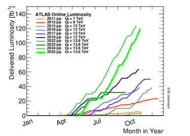
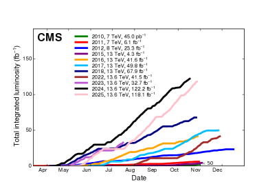
When talking about luminosity, we either refer to the instantaneous luminosity $L$ which is measured in ${\rm cm}^{-2}{\rm s}^{-1}$ or the integrated luminosity $\int L$ which is measured in ${\rm fb}^{-1}$ . An instantaneous luminosity of $L=10^{32}\,{\rm cm}^{-2}{\rm s}^{-1}$ for an entire year corresponds to $\int L=3.15\,{\rm fb}^{-1}$ .

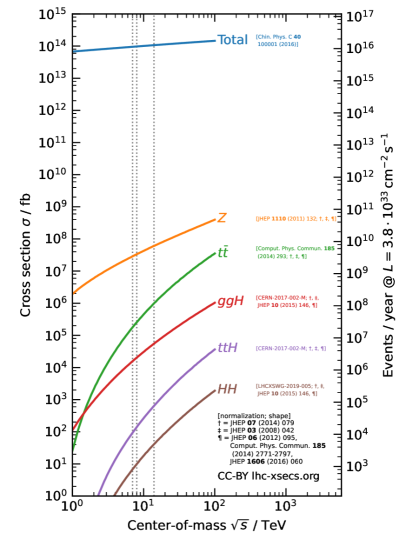
In 2024, the integrated luminosity of the LHC was around $\int_{2024}L=122.6\,{\rm fb}^{-1}$ . The LHC experiments regularly publish plots that show the luminosity recorded as a function of time over the year. The current version is reproduced in Figure 5. At the time of the Higgs discovery (summer 2012), we had only recorded about $12\,{\rm fb}^{-1}$ , slightly more than recorded in any given month. You can use the numbers for various cross sections (e.g. $\sigma(pp\to X)\approx 10^{14}\,{\rm fb}$ or $\sigma(pp\to H)\approx 5\times 10^{4}\,{\rm fb}$ ) to find the number of events expected per year. cf. Figure 5.

4.2 One initial state: decay rates

If we have only one particle in the initial state, the only interesting thing that can happen is that this particle decays. We may wonder what the lifetime $\tau$ of this particle is or, if it has multiple possible decay channels, what the relative probabilities between the channels is. To do this, we define the decay rate $\Gamma=1/\tau$ which will be larger for shorter-lived particles (i.e. those with a larger transition probability)

\displaystyle{\rm d}\Gamma=\frac{{\rm d}P_{a\to f}}{V}=\frac{1}{2M}\underbrace% {\Bigg{(}\prod_{n=1}^{f}\frac{{\rm d}^{3}p_{n}}{(2\pi)^{3}2E_{n}}\Bigg{)}(2\pi% )^{4}\delta^{(4)}\Bigg{(}p_{a}-\sum_{n=1}^{f}p_{n}\Bigg{)}}_{{\rm d}\Phi_{1\to f% }}\ \underbrace{\big{|}\langle{f}|\mathcal{T}|{a,b}\rangle\big{|}^{2}}_{|% \mathcal{M}(a\to f)|^{2}}\,,

(237)

where we have used that in the rest frame of $a$ the energy $E_{a}=M$

4.3 Examples

Let us consider a few example of this. We will use a modified version of the $\phi^{3}$ theory we discussed in the previous section that contains two fields $\phi_{1}$ and $\phi_{2}$

\displaystyle\mathcal{L}=\frac{1}{2}(\partial_{\mu}\phi_{1})(\partial^{\mu}% \phi_{1})-\frac{1}{2}M^{2}\phi_{1}^{2}+\frac{1}{2}(\partial_{\mu}\phi_{2})(% \partial^{\mu}\phi_{2})-\frac{1}{2}m^{2}\phi_{2}^{2}-\frac{1}{2!}\lambda\phi_{% 1}\phi_{2}^{2}\,.

(238)

The Feynman rules of this theory are

For each $\phi_{1}$ - $\phi_{2}$ - $\phi_{2}$ vertex	$\displaystyle=-i\lambda\,,$	(239)
For each internal $\phi_{1}$ line	$\displaystyle=\frac{i}{p^{2}-M^{2}+i\epsilon}\,,$	(240)
For each internal $\phi_{2}$ line	$\displaystyle=\frac{i}{p^{2}-m^{2}+i\epsilon}\,.$	(241)

We could have derived the Feynman rules using the Wick theorem as we did above. Alternatively, we could follow the heuristic of taking a prefactor of $-i$ , multiplying the coefficient of the fields ( $\lambda/2!$ ) and multiply with the symmetry factor ( $1!$ for the $\phi_{1}^{1}$ factor and $2!$ for the $\phi_{2}^{2}$ factor).

4.3.1 Decay process $\phi_{1}\to\phi_{2}\phi_{2}$

If we assume that $M>2m$ , the $\phi_{1}$ particle can decay into two $\phi_{2}$ particles. To do this, let us begin by calculating the matrix element $\mathcal{M}$ which is trivial in this case

\displaystyle\mathcal{M}\big{(}\phi_{1}(P)\to\phi_{2}(p_{1})\phi_{2}(p_{2})% \big{)}=\includegraphics{bmlimages/notes-133.svg}\bml@image@depth{133}% \bmlDescription{A \phi 1 particle decaying into two \phi 2 particles}\quad=-i% \lambda\,.

=−iλ.\displaystyle\mathcal{M}\big{(}\phi_{1}(P)\to\phi_{2}(p_{1})\phi_{2}(p_{2})% \big{)}=\includegraphics{bmlimages/notes-133.svg}\bml@image@depth{133}% \bmlDescription{A \phi 1 particle decaying into two \phi 2 particles}\quad=-i% \lambda\,.

(242)

The decay rate therefore is

	$\displaystyle\Gamma(\phi_{1}\to\phi_{2}\phi_{2})$	$\displaystyle=\frac{1}{2M}\int(2\pi)^{4}\delta^{(4)}\Big{(}P-p_{1}-p_{2}\Big{)% }\frac{{\rm d}^{3}p_{1}}{(2\pi)^{3}2E_{1}}\frac{{\rm d}^{3}p_{2}}{(2\pi)^{3}2E% _{2}}\|\mathcal{M}\|^{2}$		(243)
		$\displaystyle=\frac{1}{2M}\int\frac{(2\pi)\delta\Big{(}M-E_{1}-E_{2}\Big{)}}{2% E_{1}}\frac{{\rm d}^{3}p_{2}}{(2\pi)^{3}2E_{2}}\lambda^{2}\,.$		(244)

As always we have $E_{i}=\sqrt{\vec{p}_{i}^{\,2}+m^{2}}$ and since $\vec{p}_{1}=-\vec{p}_{2}$ , we have $E_{1}=E_{2}$ . We can now write the ${\rm d}^{3}p_{2}$ integration in spherical coordinates, i.e. ${\rm d}^{3}p_{2}=|\vec{p}_{2}|^{2}{\rm d}|\vec{p}_{2}|{\rm d}\Omega$

\displaystyle\Gamma(\phi_{1}\to\phi_{2}\phi_{2})

\displaystyle=\frac{1}{2M}\int\frac{(2\pi)\delta\big{(}M-2E_{2}\big{)}}{4E_{2}% ^{2}}\frac{{\rm d}\Omega|\vec{p}_{2}|^{2}{\rm d}|\vec{p}_{2}|}{(2\pi)^{3}}% \lambda^{2}\,.

(245)

Since there is no angular dependence, we can solve the ${\rm d}\Omega$ integral and obtain $4\pi$ . To solve the ${\rm d}|\vec{p}_{2}|$ integration, we can perform a substitution ${\rm d}|\vec{p}_{2}|={\rm d}E_{2}\times E_{2}/\sqrt{E_{2}^{2}-m^{2}}$

\displaystyle\Gamma(\phi_{1}\to\phi_{2}\phi_{2})

\displaystyle=\frac{\lambda^{2}}{8\pi}\int\frac{{\rm d}E_{2}}{E_{2}}\frac{% \sqrt{E_{2}^{2}-m^{2}}}{M}\delta(M-2E_{2})=\frac{\lambda^{2}}{16\pi M}\sqrt{1-% 4m^{2}/M^{2}}\,.

(246)

We can identify $\sqrt{1-4m^{2}/M^{2}}$ as the velocity of one of the $\phi_{2}$ particles since it is defined as

\displaystyle\beta=\frac{|\vec{p}_{1}|}{E_{1}}=\sqrt{1-\frac{m^{2}}{E_{1}^{2}}% }=\sqrt{1-\frac{4m^{2}}{M^{2}}}\,,

(247)

with $E_{1}=M/2$ .

Suggested Exercise

Can you explain why we required $M>2m$ based on this answer? What happens to $\beta$ for $M<2m$ , for $M=2m$ or for $M\gg 2m$ ?

The region $M=2m$ is referred to as the threshold where the decay is just about possible and the two final-state particles are produced at rest.

Suggested Exercise

The decay $\phi_{1}\to\phi_{2}\phi_{2}\phi_{2}\phi_{2}$ is also possible. How would you go about calculating this? The first Feynman diagram would be

\displaystyle\includegraphics{bmlimages/notes-134.svg}\bml@image@depth{134}% \bmlDescription{A \phi 1 particle decaying into two \phi 2 particles. One of % the \phi 2 emits another \phi 1 which again decays into another pair of \phi 2% }\quad=(-i\lambda)\frac{i}{(P-p_{4})^{2}-m^{2}+i\epsilon}(-i\lambda)\frac{i}{(% p_{2}+p_{3})^{2}-M^{2}+i\epsilon}\,.

A ϕ1 particle decaying into two ϕ2 particles. One of the ϕ2 emits another ϕ1 which again decays into another pair of ϕ2

=(−iλ)i(P−p4)2−m2+i⁢ϵ(−iλ)i(p2+p3)2−M2+i⁢ϵ.\displaystyle\includegraphics{bmlimages/notes-134.svg}\bml@image@depth{134}% \bmlDescription{A \phi 1 particle decaying into two \phi 2 particles. One of % the \phi 2 emits another \phi 1 which again decays into another pair of \phi 2% }\quad=(-i\lambda)\frac{i}{(P-p_{4})^{2}-m^{2}+i\epsilon}(-i\lambda)\frac{i}{(% p_{2}+p_{3})^{2}-M^{2}+i\epsilon}\,.

(248)

There are more diagrams due to the permutations of the outgoing particles. Convince yourself of the above and calculate the full amplitude.

More generally, it is useful to keep

\displaystyle\int{\rm d}\Phi_{2}=\int{\rm d}\Omega\frac{1}{16\pi^{2}}\frac{|% \vec{p}_{1}|}{E_{\rm cm}}

(249)

in mind. Here $E_{\rm cm}=M$ and the ${\rm d}\Omega$ integral was trivial.

4.3.2 Scattering of $\phi_{2}\phi_{2}\to\phi_{2}\phi_{2}$

Let us now calculate the scattering of two $\phi_{2}$ particles. The amplitude $\mathcal{M}$ contains three diagrams

$\displaystyle\mathcal{M}\big{(}\phi_{2}(p_{1})$	$\displaystyle\phi_{2}(p_{2})\to\phi_{2}(p_{3})\phi_{2}(p_{4})\big{)}=% \includegraphics{bmlimages/notes-135.svg}\bml@image@depth{135}\bmlDescription{% Two \phi 2 particles (p1 and p2) annihilating into a \phi 1 particle which % then decays into two \phi 2 (p3 and p4)}+\includegraphics{bmlimages/notes-136.% svg}\bml@image@depth{136}\bmlDescription{Two \phi 2 particles (p1 and p2) % scattering through a \phi 1 particle. This is the rotated version of the % previous diagram}+\includegraphics{bmlimages/notes-137.svg}\bml@image@depth{13% 7}\bmlDescription{Same as previous but p3 and p4 are flipped}$ + + \displaystyle\phi_{2}(p_{2})\to\phi_{2}(p_{3})\phi_{2}(p_{4})\big{)}=% \includegraphics{bmlimages/notes-135.svg}\bml@image@depth{135}\bmlDescription{% Two \phi 2 particles (p1 and p2) annihilating into a \phi 1 particle which % then decays into two \phi 2 (p3 and p4)}+\includegraphics{bmlimages/notes-136.% svg}\bml@image@depth{136}\bmlDescription{Two \phi 2 particles (p1 and p2) % scattering through a \phi 1 particle. This is the rotated version of the % previous diagram}+\includegraphics{bmlimages/notes-137.svg}\bml@image@depth{13% 7}\bmlDescription{Same as previous but p3 and p4 are flipped}	(250)
	$\displaystyle=(-i\lambda)\frac{i}{(p_{1}+p_{2})^{2}-M^{2}}(-i\lambda)+(-i% \lambda)\frac{i}{(p_{1}-p_{3})^{2}-M^{2}}(-i\lambda)+(-i\lambda)\frac{i}{(p_{1% }-p_{4})^{2}-M^{2}}(-i\lambda)$
	$\displaystyle=-i\lambda^{2}\bigg{(}\frac{1}{s-M^{2}}+\frac{1}{t-M^{2}}+\frac{1% }{u-M^{2}}\bigg{)}\,.$	(251)

Here we have defined the Mandelstam variables

\displaystyle s=(p_{1}+p_{2})^{2}=(p_{3}+p_{4})^{2}\,,\quad t=(p_{1}-p_{3})^{2% }=(p_{2}-p_{4})^{2}\,,\quad u=(p_{1}-p_{4})^{2}=(p_{2}-p_{3})^{2}\,.

(252)

Suggested Exercise

Use momentum conservation to show that $s+t+u=4m^{2}$ .

The Lorentz-invariant phase space is calculated the same way as before

\displaystyle\int{\rm d}\Phi_{2\to 2}=\int\frac{{\rm d}^{3}p_{3}}{(2\pi)^{3}2E% _{3}}\frac{{\rm d}^{3}p_{4}}{(2\pi)^{3}2E_{4}}(2\pi)^{4}\delta^{(4)}\Big{(}p_{% 1}+p_{2}-p_{3}-p_{4}\Big{)}=\int{\rm d}\Omega\frac{1}{16\pi^{2}}\frac{|\vec{p}% _{3}|}{E_{\rm cm}}\,,

(253)

with $E_{\rm cm}=E_{1}+E_{2}$ . Unfortunately we now cannot replace ${\rm d}\Omega=4\pi$ because we still have an angular dependency. To see why, let us write down explicit four vectors in the centre-of-mass frame where $\vec{p}_{1}+\vec{p}_{2}=0$ . For simplicity, we align our coordinate system such that the beam axis is the $z$ direction and that the scattering takes place in the $y$ - $z$ plane

$\displaystyle p_{1}$	$\displaystyle=$	$\displaystyle\big{(}E,0,0,+\|\vec{p}_{1}\|\big{)}$	$\displaystyle=$	$\displaystyle\big{(}E,0,0,+\sqrt{E^{2}-m^{2}}\big{)}\,,$	(254)
$\displaystyle p_{2}$	$\displaystyle=$	$\displaystyle\big{(}E,0,0,-\|\vec{p}_{2}\|\big{)}$	$\displaystyle=$	$\displaystyle\big{(}E,0,0,-\sqrt{E^{2}-m^{2}}\big{)}\,,$	(255)
$\displaystyle p_{3}$	$\displaystyle=$	$\displaystyle\big{(}E,0,+\sin\theta\|\vec{p}_{3}\|,+\cos\theta\|\vec{p}_{3}\|\big{)}$	$\displaystyle=$	$\displaystyle\big{(}E,0,+\sin\theta\sqrt{E^{2}-m^{2}},+\cos\theta\sqrt{E^{2}-m% ^{2}}\big{)}\,,$	(256)
$\displaystyle p_{4}$	$\displaystyle=$	$\displaystyle\big{(}E,0,-\sin\theta\|\vec{p}_{4}\|,-\cos\theta\|\vec{p}_{4}\|\big{)}$	$\displaystyle=$	$\displaystyle\big{(}E,0,-\sin\theta\sqrt{E^{2}-m^{2}},-\cos\theta\sqrt{E^{2}-m% ^{2}}\big{)}\,.$	(257)

Since $E\equiv E_{1}=\sqrt{|\vec{p}_{1}|^{2}-m^{2}}=E_{2}$ . For the same reason, $\vec{p}_{3}+\vec{p}_{4}=0$ and $E_{3}=E_{4}$ . The Mandelstam variables are


$\displaystyle s$	$\displaystyle=\big{(}2E,0,0,0\big{)}^{2}=4E^{2}=E_{\rm cm}^{2}\,,$	(258a)
$\displaystyle t$	$\displaystyle=\big{(}0,0,-\sin\theta,(+1-\cos\theta)\big{)}^{2}(E^{2}-m^{2})=-% 2(E^{2}-m^{2})(1-\cos\theta)\,,$	(258b)
$\displaystyle u$	$\displaystyle=\big{(}0,0,+\sin\theta,(-1-\cos\theta)\big{)}^{2}(E^{2}-m^{2})=-% 2(E^{2}-m^{2})(1+\cos\theta)\,.$	(258c)

We can now write the differential cross section as

	$\displaystyle{\rm d}\sigma$	$\displaystyle=\frac{1}{(2E)^{2}\|\vec{v}\|}\frac{{\rm d}\Omega}{16\pi^{2}}\frac{% \sqrt{E^{2}-m^{2}}}{2E}\lambda^{4}\bigg{(}\frac{1}{s-M^{2}}+\frac{1}{t-M^{2}}+% \frac{1}{u-M^{2}}\bigg{)}^{2}$		(259)
		$\displaystyle=\frac{{\rm d}\Omega}{64\pi^{2}}\frac{\lambda^{4}}{E^{2}(M^{2}-4E% ^{2})^{2}}\Bigg{(}\frac{14E^{4}-2m^{4}+4m^{2}(2M^{2}-3E^{2})-3M^{4}+2(m^{2}-E^% {2})^{2}\cos(2\theta)}{(2E^{2}-2m^{2}+M^{2})^{2}-4(m^{2}-E^{2})^{2}\cos^{2}% \theta}\Bigg{)}^{2}\,.$		(260)

If we set $M=m=0$ , we find a very short expression

\displaystyle{\rm d}\sigma=\frac{{\rm d}\Omega}{1024\pi^{2}}\frac{\lambda^{4}}% {E^{6}}\frac{(3+\cos^{2}\theta)^{2}}{(1-\cos^{2}\theta)^{2}}\,.

(261)

What do we now do with this object? We can either visualise the differential distribution ${\rm d}\sigma/{\rm d}\Omega$ , normally written as ${\rm d}\sigma/{\rm d}(\cos\theta)$ or ${\rm d}\sigma/{\rm d}\theta$ . Alternatively, we could integrate over ${\rm d}\Omega$ and obtain the full cross section of this process occurring.

A few comments are in-order. From (258) it is clear that $s=4E^{2}\geq 4m^{2}>0$ and $t,u\leq 0$ . This means the second and third term in (259) will not be a problem as long $M\neq 0$ . However, $s=M^{2}$ is allowed and the cross section would explode if we picked this value of $s$ . This is fixed by adding higher-order corrections to the $\phi_{1}$ propagator, i.e.

\displaystyle\includegraphics{bmlimages/notes-138.svg}\bml@image@depth{138}+% \includegraphics{bmlimages/notes-139.svg}\bml@image@depth{139}+% \includegraphics{bmlimages/notes-140.svg}\bml@image@depth{140}+\cdots\,.

+⋯.\displaystyle\includegraphics{bmlimages/notes-138.svg}\bml@image@depth{138}+% \includegraphics{bmlimages/notes-139.svg}\bml@image@depth{139}+% \includegraphics{bmlimages/notes-140.svg}\bml@image@depth{140}+\cdots\,.

(262)

Even though each term is progressively more suppressed by $\lambda$ , the addition of more propagators $1/(s-M^{2})$ makes up for this and we need to calculate infinitely many such insertions. We will come back to this in Section 7 and Appendix A.

We should also note the behaviour of (261) for $\cos\theta\to\pm 1$ . This corresponds to a scattering angle of $\theta=0$ or $\theta=\pi$ , i.e. when the outgoing particles follow the beam axis. Since the two $\phi_{2}$ particles are indistinguishable, this just means that the particles pass each other without interacting. The divergence we see here is to the fact that we have split the $\mathcal{S}$ matrix as $\mathcal{S}=1+\mathcal{T}$ in (227). When we constructed $\mathcal{T}$ we assumed that the initial and final state were different which is not the case for $\cos\theta=\pm 1$ .

4 Cross sections and decay rates

4.1 Two initial states: cross section

4.2 One initial state: decay rates

4.3 Examples

4.3.1 Decay process ϕ1→ϕ2⁢ϕ2\phi_{1}\to\phi_{2}\phi_{2}

4.3.2 Scattering of ϕ2⁢ϕ2→ϕ2⁢ϕ2\phi_{2}\phi_{2}\to\phi_{2}\phi_{2}

4.3.1 Decay process $\phi_{1}\to\phi_{2}\phi_{2}$

4.3.2 Scattering of $\phi_{2}\phi_{2}\to\phi_{2}\phi_{2}$