Computerised calculation of

In this Mathematica notebook, I will demonstrate how to use computers to calculate . This supplements the calculation in Section 6.3 of my QFT lecture notes and uses the same notation etc. The goal of this notebook is to demonstrate that these calculations can be fully automatised, at least as long as there are no loops are involved.

This notebook runs through on my Linux laptop where I have installed all dependencies. If you want to run this on your own laptop, please install Package X by downloading this zip file and uncompressing it in your $UserBaseDirectory/Applications/ directory. Please also download the file qgraf.wl into the same directory.

To find this folder, you can execute the following code block

Installing the diagram generator is more complicated and will not be part of this example.

Load Package X and QGraf

Once you have installed Package X and qgraf.wl we can load it here. Note that this will fail if you have not installed it correct.

Following the recipe

Step 1-4: generating the amplitude

For the first four steps

Draw all Feynman diagrams.

assign momenta to all edges and Lorentz indices to all photon vertices

pick the end of any fermion line and follow the arrow backwards, evaluating as you go

multiply in the polarisation tensors for any external photons and propagators for each internal photon

We can use the diagram generator QGraf. Note that this section of the code has been disabled to avoid accidental deletion

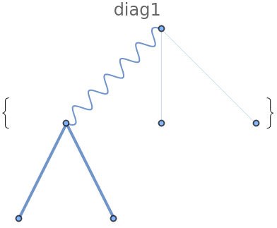
As you can see, the code has generated the diagram we were after using the correct spinors but has dropped a factor of i. Since we will calculate this would drop out anyway. Also, note that the code has picked momenta labels for incoming and for outgoing momenta as well as ‘random’ Lorentz indices.

Please note that Package-X uses always lower indices. This is not formally correct but simplifies the notation and it can always be mapped on the more correct notation.

Step 5-7: finishing the amplitude

Let us relabel the outgoing momenta to match the lecture notes

contract any open index

if your diagram has any loops, integrate over the unconstrained momenta. If you have any internal fermion loops, calculate the trace over their gamma matrices.

Since we have no loops to integrate, we do nothing

you now have the amplitude M

Steps 8-10: squaring the amplitude

We can perform these operations manually or we use the function FermionSpinSum to perform steps 8-10

square the amplitude as

Note how we have now introduced the index to avoid collisions!

if you calculate unpolarised scattering, sum over final-state and average over initial-state polarisations.

for fermions, this will result in a trace of γ matrices

We can now contract the open indices to write terms of scalar products.

We could express this in terms of s, t, u using

Kinematics

If we want to calculate for example, dσ/dΩ it would be better to write this in terms of cosθ and φ. To do this, let us define the scalar product as

and parameterise our momenta (here we once again use a function that is not part of the normal Mathematica suite, therefore the following block is disabled).

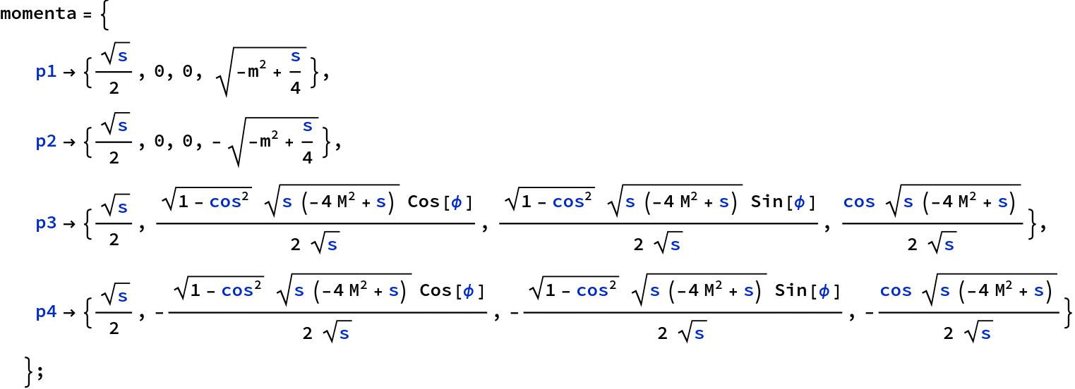
We can verify that , , and

More importantly, we can calculate

Our matrix element can be written as

The velocity of the muon is defined as

Step 11-12: cross section

We can now calculate the cross section as

calculate the cross section as

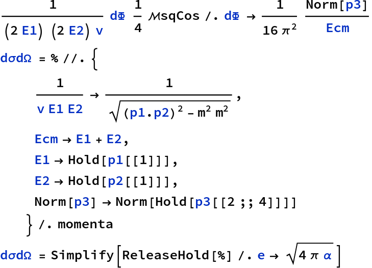
Using what we know about the phase space

We have

In the lecture we then set m=0 and identified the velocity of the muon β

We can now set for example the muon mass to zero, i.e. β=1

or calculate the total cross section

integrate over phase space

Plots

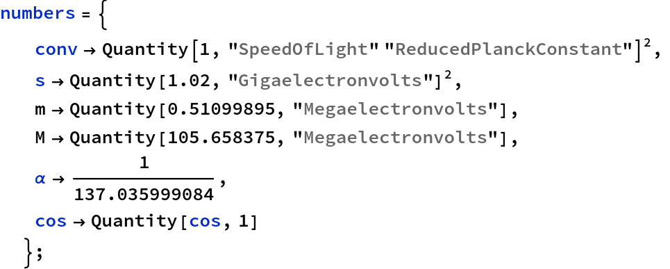
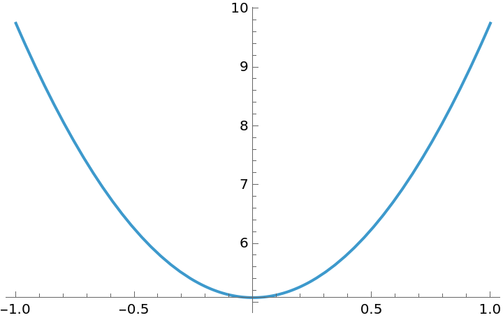
We can now show our result. For example at the KLOE experiment which has , we have

Going beyond the lecture (not examinable)

We can also calculate the one-loop corrections to this.

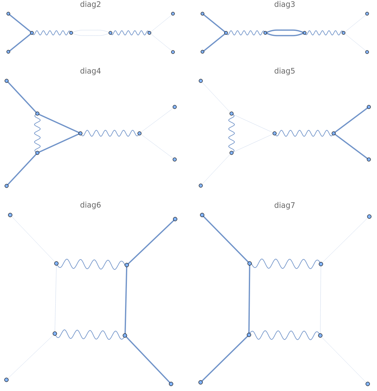
Note that we now have both closed fermion loops (first row of diagrams) and unconstrained momenta. The generator chose a specific routing for us, i.e. it identified a momentum to be the loop momentum . We can use the technology we are developing in Chapter 7 to calculate this in dimensional regularisation

Export for the web